
Class Project
AA-548 Linear Multivariable Control 📡
Spring 2025
- Implemented a cascaded PID controller for a 12 state quadrotor dynamical system.
- Developed control augmentation to baseline controller using Control Barrier Functions to enforce pitch attitude constraints.
- Investigated standard and Higher-Order CBFs for enforcing safety on second order dynamical system such as quadrotor.
🛰 Safe Control using Control Barrier Functions 🛩️
Theory
Modern safety-critical systems require integrated decision-making, planning, and control frameworks to accomplish mission objectives while ensuring operational safety. Control Barrier Functions (CBFs) have emerged as a valuable strategy for synthesizing controllers to ensure that state or output constraints are satisfied during system evolution. CBFs explicitly incorporate the control input into their formulation, ensuring the states remain within a predefined safe set and thus enforce safety.
Let \( h:\mathbb{R}^n \rightarrow \mathbb{R} \) be a scalar function, and suppose we have control affine dynamics \( \dot{x} = f(x,u) \). Define the safe set as \( \mathcal{S} = \{ x \mid h(x) \geq 0\} \). Then \( h \) is a CBF for the system \( \dot{x} = f(x,u) \) if there exists a class \( \mathcal{K} \) function \( \alpha \) such that:\[ \max_{u\in\mathcal{U}} \nabla h(x)^Tf(x,u) \geq -\alpha(h(x)) , \quad \forall \: x\in\mathcal{S} \]
\( -\alpha(h(x)) \) provides the behavior we want where we gradually restrict the motion of the system as it approaches the boundary of \( \mathcal{S}\). The max operation there is to ensure that there exists at least one control that satisfies the inequality. If we can find a function that satisfy the inequality over the domain, then we can guarantee that if the system starts inside \( \mathcal{S}\), then it will remain inside \( \mathcal{S}\) for all future time.Hence, to ensure the system remains inside \( \mathcal{S} \), we need to guarantee that the control input satisfies this inequality at all times. This trade-off can be formulated as an optimization problem:
\[ u^\star = \underset{u}{\text{argmin}} \; \| u - u_{\mathrm{nom}} \|_2^2 \] \[ \text{subject to} \quad \nabla h(x)^T f(x,u) \geq -\alpha(h(x)) \]
For systems with control-affine dynamics, this optimization problem becomes a Quadratic Program (QP), which is a convex optimization problem that can be solved efficiently using standard solvers.
Quadrotor Dynamics
Quadcopter is an underactuated aircraft powered by four rotors to lift off and controlled by varying the motor speed of each rotor, thus altering the generated lift to perform roll, pitch, and yaw. [1].
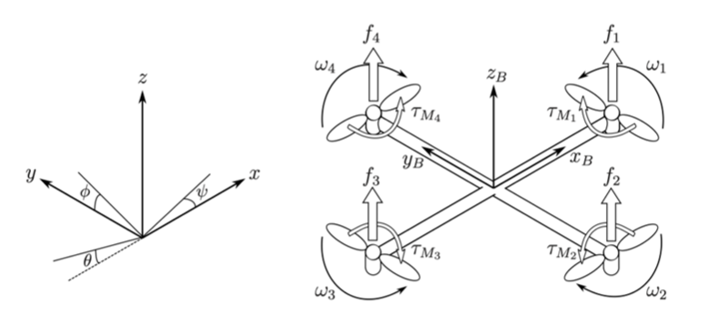
Figure 1: Forces & Moments Acting on the Quadcopter
Equations of Motion:
\[ \ddot{x} = \frac{T}{m} \left( \cos\psi \sin\theta \cos\phi + \sin\psi \sin\phi \right) \] \[ \ddot{y} = \frac{T}{m} \left( \sin\psi \sin\theta \cos\phi - \cos\psi \sin\phi \right) \] \[ \ddot{z} = \frac{T}{m} \cos\theta \cos\phi - g \] \[ \ddot{\phi} = \frac{k l}{I_x} \left(-\omega_1^2 + \omega_2^2 + \omega_3^2 - \omega_4^2 \right) c \] \[ \ddot{\theta} = \frac{k l}{I_y} \left(-\omega_1^2 - \omega_2^2 + \omega_3^2 - \omega_4^2 \right) c \] \[ \ddot{\psi} = \frac{b}{I_z} \left(\omega_1^2 - \omega_2^2 + \omega_3^2 - \omega_4^2 \right) \] where, the states and controls are:States:
\[
\mathbf{x} = [x,\, y,\, z,\, \phi,\, \theta,\, \psi,\, \dot{x},\, \dot{y},\, \dot{z},\, \dot{\phi},\, \dot{\theta},\, \dot{\psi}]^\top
\]
Controls Inputs:
\[
\mathbf{u} = [
\omega_1,\, \omega_2,\, \omega_3,\, \omega_4,\, T]
\]
Controls Inputs:
\[ \mathbf{u} = [ \omega_1,\, \omega_2,\, \omega_3,\, \omega_4,\, T] \]The nonlinear dynamics are linearized about a hover point condition to obtain the linear state space representation of the form:
\[ \dot{x} = A x + B u \]
\[ y = C x + D u \]
Our objective is to design a controller for the above system that keeps the pitch within some defined limits. \[ \theta_{\min} \leq \theta \leq \theta_{\max} \]PID Tracking Controller
A tracking PID controller is designed to follow a reference pitch trajectory and reference Vz speed.\[ \theta_{commanded} = 0.3 \cdot \sin(0.2 \cdot t) \] \[ Vz = 0.1 \]
Figure 2. shows the states time history when commanding the pitch reference trajectory and Vz, using the PID controller with Initial Conditions: \[ \mathbf{x} = \begin{bmatrix} 1 & 0 & 1 & 0 & 0 & 0 & 0 & 0 & 0 & 0 & 0 & 0 \end{bmatrix}^\top \]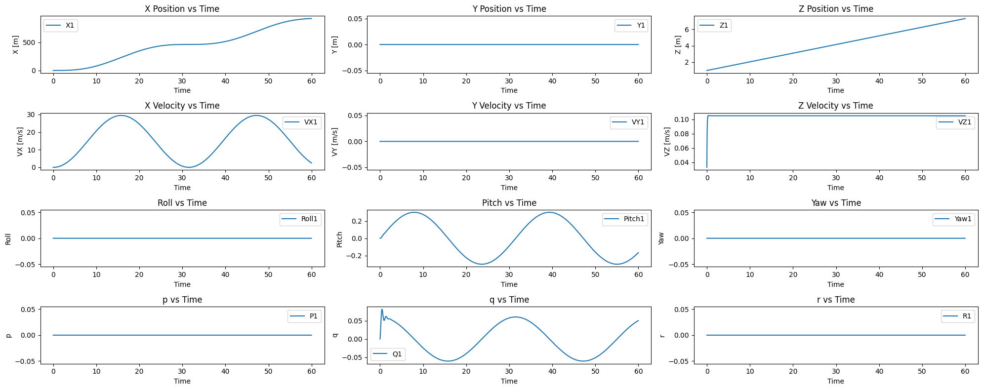
Figure 2: States time history using PID controller
Traditional CBF Approach
An initial approach to enforce pitch constraints involved implementing a candidate quadratic Control Barrier Function (CBF) of the form \( h(\theta) = (\theta - \theta_{\min})(\theta_{\max} - \theta) \), intended to maintain pitch within specified bounds. However, simulation results indicated that this method had no noticeable effect on limiting the pitch angle.
This limitation arises due to the relative degree of the CBF with respect to the system dynamics — specifically, the fact that the control input influence is not directly affecting the pitch state \( \theta\), but the pitch rate state \( \dot{\theta}\).
To address this, we will explore higher-order CBFs (HOCBFs), enabling the enforcement of safety constraints on pitch more effectively.
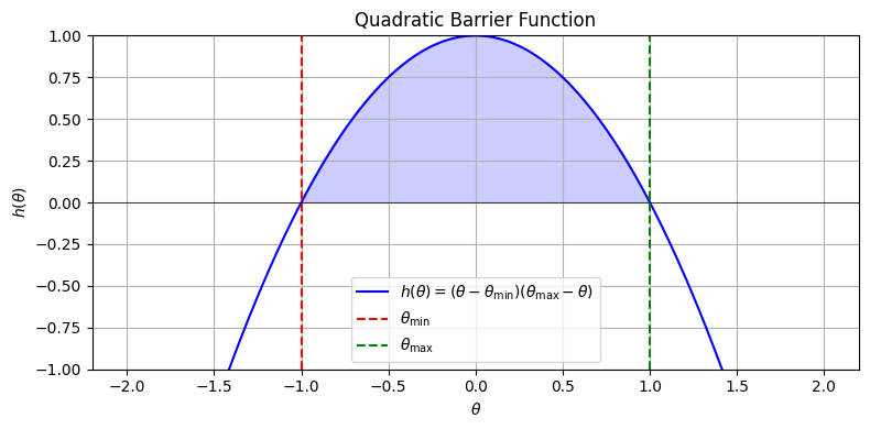
Figure 3: Candidate CBF \( h(x) \geq 0\ \)
High Order CBF Approach
To address the limitation imposed by the relative degree of the pitch constraint, we leverage the use of a Higher-Order Control Barrier Function (HOCBF), originally used by Authors in [2] for a Pendulum case. The HOCBF is useful to enforce a safe pitch range by including both the pitch angle \( \theta \) and its derivative \( \dot{\theta} \), allowing direct influence over the control input. The candidate function is defined as:
\[ h(\mathbf{x}) = \bar{\theta}^2 - \theta^2 - \frac{1}{2}(\dot{\theta} + \theta)^2 \]
This formulation not only penalizes deviations of \( \theta \) from the allowable bounds \( \pm \bar{\theta} \), but also incorporates the pitch rate \( \dot{\theta} \), discouraging fast pitch movements that could lead to constraint violations in the near future.
The gradients of this barrier function with respect to the states are:
\[ \nabla h_{\theta} = \frac{\partial h}{\partial \theta} = -3\theta - \dot{\theta} \] \[ \nabla h_{\dot{\theta}} = \frac{\partial h}{\partial \dot{\theta}} = -(\dot{\theta} + \theta) \]
Because the gradient \( \nabla h_{\dot{\theta}} \) explicitly depends on \( \dot{\theta} \), which is dynamically coupled to the control input through the system equations (e.g., torque input in a quadrotor), this HOCBF is capable of shaping the control action to enforce the pitch constraint in a proactive manner.
This approach circumvents the challenge of a relative degree greater than one by leveraging Lie derivatives of the barrier function up to the second order. As such, it is expected to produce a feasible control action that respects the pitch bounds while maintaining system stability. From Figure 4. we can see that implementing the HOCBF constraint to synthetize the control input, we are able to keep the quadcopter within the bounds of \( -0.2 \leq \theta \leq +0.2\)
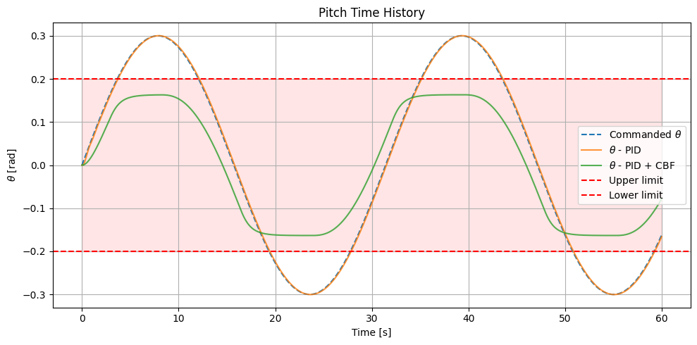
Figure 4: Pitch time history using PID + HOCBF
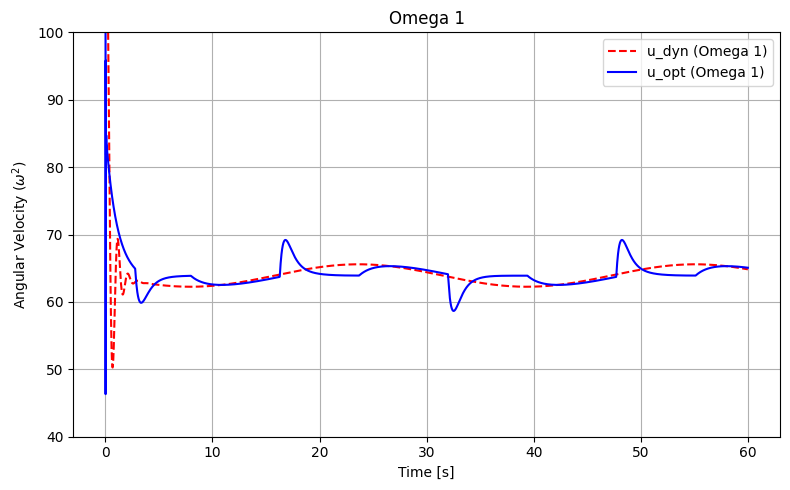
Figure 5: Angular rate in \( \omega_1 \)
Takeaways
- Traditional Control Barrier Functions (CBFs) may fail to enforce constraints effectively in systems with high relative degree, where the safety constraint does not appear directly in the first derivative of the state.
- Higher-Order Control Barrier Functions (HOCBFs) extend the applicability of CBFs by handling such high-relative-degree constraints, enabling direct influence over the control input.
- Incorporating HOCBFs into a Quadratic Programming (QP) optimization framework allows for the systematic computation of control inputs that balance performance with safety, which is critical in real-time, safety-critical systems like autonomous drones or vehicles.
- The proposed method demonstrates potential for practical applications, such as maintaining pitch limits to ensure stable flight.
References:
- Budihartono, Michael, "In-Flight Testing & Verification of an Adaptive Distributed Fault-Tolerant Control Architecture" (2023). Doctoral Dissertations and Master's Theses. 753.
- Cohen, M. H., Molnar, T. G., and Ames, A. D., "Safety-critical control for autonomous systems: Control barrier functions via reduced-order models," (2024). Annual Reviews in Control, Vol. 57, pp. 100947
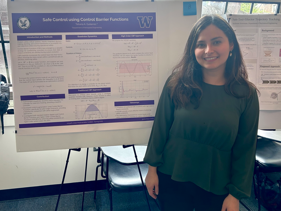
Poster presentation @UW, June 2025